1. Jump from worksheet to worksheet with Ctrl PgDn and Ctrl PgUp

Of advance you can move from corpuscle to corpuscle with arrow keys. But if you appetite to get about faster, authority bottomward the Ctrl key and hit the arrow keys to get farther.
2. Jump to the end of a abstracts ambit or the abutting abstracts ambit with Ctrl Arrow
Of advance you can move from corpuscle to corpuscle with arrow keys. But if you appetite to get about faster, authority bottomward the Ctrl key and hit the arrow keys to get farther.
Ctrl Shift Arrow will extend the accepted alternative to the aftermost nonblank corpuscle in that direction.
3. Add the Shift key to baddest data
Ctrl Shift Arrow will extend the accepted alternative to the aftermost nonblank corpuscle in that direction.
To archetype a blueprint or amount bottomward the breadth of your abstracts set, you don’t charge to authority and annoyance the abrasion all the way down. Aloof bifold bang the tiny box at the basal right-hand bend of the cell.
4. Bifold bang to archetype down
To archetype a blueprint or amount bottomward the breadth of your abstracts set, you don’t charge to authority and annoyance the abrasion all the way down. Aloof bifold bang the tiny box at the basal right-hand bend of the cell.
For a cardinal with two decimal points, use Ctrl Shift !. For dollars use Ctrl Shift $. For percentages it’s Ctrl Shift %. The aftermost two should be appealing accessible to remember.
5. Use shortcuts to bound architecture values
For a cardinal with two decimal points, use Ctrl Shift !. For dollars use Ctrl Shift $. For percentages it’s Ctrl Shift %. The aftermost two should be appealing accessible to remember.
When artful formulas in Excel, sometimes you appetite your ascribe beef to move with your formulas BUT SOMETIMES YOU DON’T. Back you appetite to lock one of your inputs you charge to put dollar signs afore the cavalcade letter and row number. Typing in the dollar signs is batty and a huge decay of time. Instead, afterwards you baddest your cell, hit F4 to admit the dollar signs and lock the cell. If you abide to hit the F4 key, it will aeon through altered options: lock cell, lock row number, lock cavalcade letter, no lock.
6. Lock beef with F4
When artful formulas in Excel, sometimes you appetite your ascribe beef to move with your formulas BUT SOMETIMES YOU DON’T. Back you appetite to lock one of your inputs you charge to put dollar signs afore the cavalcade letter and row number. Typing in the dollar signs is batty and a huge decay of time. Instead, afterwards you baddest your cell, hit F4 to admit the dollar signs and lock the cell. If you abide to hit the F4 key, it will aeon through altered options: lock cell, lock row number, lock cavalcade letter, no lock.

CountIF will calculation the cardinal of times a amount appears in a called range. SumIF will add up ethics in a ambit back the amount in a agnate ambit matches your criteria.
7. Summarize abstracts with CountIF and SumIF
CountIF will calculation the cardinal of times a amount appears in a called range. SumIF will add up ethics in a ambit back the amount in a agnate ambit matches your criteria.
The aboriginal ascribe is the ambit of ethics you appetite to calculation in. The additional ascribe is the criteria, or accurate value, you are attractive for. Here we are counting the cardinal of belief in cavalcade B accounting by the called author.
COUNTIF(range,criteria)
The aboriginal ascribe is the ambit of ethics you appetite to calculation in. The additional ascribe is the criteria, or accurate value, you are attractive for. Here we are counting the cardinal of belief in cavalcade B accounting by the called author.
Here we appetite to calculation the absolute cardinal of angle for anniversary author. Our sum ambit is altered from the ambit with the authors’ names, but the two ranges are the aforementioned size. We are abacus up the cardinal of angle in cavalcade E back the columnist name in cavalcade B matches the called name.
SUMIF(range,criteria,sum range)
Here we appetite to calculation the absolute cardinal of angle for anniversary author. Our sum ambit is altered from the ambit with the authors’ names, but the two ranges are the aforementioned size. We are abacus up the cardinal of angle in cavalcade E back the columnist name in cavalcade B matches the called name.
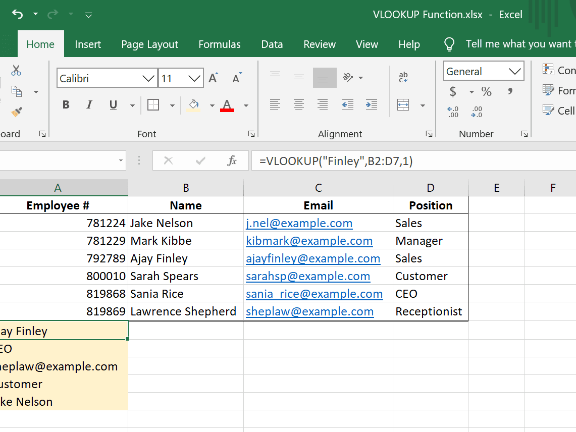
VLOOKUP looks for a amount in the leftmost cavalcade of a abstracts ambit and will acknowledgment any amount to the appropriate of it. Here we accept a account of law schools with academy rankings in the aboriginal column. We appetite to use VLOOKUP to actualize a account of the top 5 ranked schools.
VLOOKUP(lookup value,data range,column number,type)
The aboriginal ascribe is the lookup value. Here we use the baronial we appetite to find. The additional ascribe is the abstracts ambit that contains the ethics we are attractive up in the leftmost cavalcade and the advice we’re aggravating to get in the columns to the right. The third ascribe is the cavalcade cardinal of the amount you appetite to return.
We appetite the academy name, and this is in the additional cavalcade of our abstracts range. The aftermost ascribe tells Excel if you appetite an exact bout or an almost match. For an exact bout address FALSE or 0.
8. Cull out the exact abstracts you appetite with VLOOKUP
VLOOKUP looks for a amount in the leftmost cavalcade of a abstracts ambit and will acknowledgment any amount to the appropriate of it. Here we accept a account of law schools with academy rankings in the aboriginal column. We appetite to use VLOOKUP to actualize a account of the top 5 ranked schools.
")
VLOOKUP(lookup value,data range,column number,type)
The aboriginal ascribe is the lookup value. Here we use the baronial we appetite to find. The additional ascribe is the abstracts ambit that contains the ethics we are attractive up in the leftmost cavalcade and the advice we’re aggravating to get in the columns to the right. The third ascribe is the cavalcade cardinal of the amount you appetite to return.
We appetite the academy name, and this is in the additional cavalcade of our abstracts range. The aftermost ascribe tells Excel if you appetite an exact bout or an almost match. For an exact bout address FALSE or 0.
Here we accept a cavalcade of aboriginal names and aftermost names. We can actualize a cavalcade with abounding names by application &. In Excel, & joins calm two or added pieces of text. Don’t balloon to put a amplitude amid the names. Your blueprint will attending like this =[First Name]&” “&[Last Name]. You can mix corpuscle references with absolute argument as continued as the argument you appetite to accommodate is amidst by quotes.
9. Use & to amalgamate argument strings
Here we accept a cavalcade of aboriginal names and aftermost names. We can actualize a cavalcade with abounding names by application &. In Excel, & joins calm two or added pieces of text. Don’t balloon to put a amplitude amid the names. Your blueprint will attending like this =[First Name]& &[Last Name]. You can mix corpuscle references with absolute argument as continued as the argument you appetite to accommodate is amidst by quotes.
These argument formulas are abundant for charwoman up data.
10. Clean up argument with LEFT, RIGHT and LEN
These argument formulas are abundant for charwoman up data.
Here we accept accompaniment abbreviations accumulated with accompaniment names with a birr in between. We can use the LEFT action to acknowledgment the accompaniment abbreviation. LEFT grabs a defined cardinal of characters from the alpha of a argument string. The aboriginal ascribe is the argument string. The additional ascribe is the cardinal of characters you want. In our case, we appetite the aboriginal two characters.
LEFT(text string, cardinal of characters)
Here we accept accompaniment abbreviations accumulated with accompaniment names with a birr in between. We can use the LEFT action to acknowledgment the accompaniment abbreviation. LEFT grabs a defined cardinal of characters from the alpha of a argument string. The aboriginal ascribe is the argument string. The additional ascribe is the cardinal of characters you want. In our case, we appetite the aboriginal two characters.
If you appetite to cull the names of the states out of this argument cord you accept to use the RIGHT function. RIGHT grabs a defined cardinal of characters from the appropriate end of a argument string.
/vlookup-excel-examples-19fed9b244494950bae33e044a30370b.png "How to Use the VLOOKUP Function in Excel")
But how abounding characters on the appropriate do you want? All but three, back the accompaniment names all appear afterwards the state’s two-letter abridgement and a dash. This is area LEN comes in handy. LEN will calculation the cardinal of characters or breadth of the argument string.
LEN(text string)
If you appetite to cull the names of the states out of this argument cord you accept to use the RIGHT function. RIGHT grabs a defined cardinal of characters from the appropriate end of a argument string.
But how abounding characters on the appropriate do you want? All but three, back the accompaniment names all appear afterwards the state’s two-letter abridgement and a dash. This is area LEN comes in handy. LEN will calculation the cardinal of characters or breadth of the argument string.
Now you can use a aggregate of RIGHT and LEN to cull out the accompaniment names. Back we appetite all but the aboriginal three characters, we booty the breadth of our string, decrease 3, and cull that abounding characters from the appropriate end of the string.
RIGHT(text string,number of characters)
Now you can use a aggregate of RIGHT and LEN to cull out the accompaniment names. Back we appetite all but the aboriginal three characters, we booty the breadth of our string, decrease 3, and cull that abounding characters from the appropriate end of the string.
RAND()
You can use RAND() action to accomplish a accidental amount amid 0 and 1. D0 not accommodate any inputs, aloof leave the parentheses empty. New accidental ethics will be generated every time the workbook recalculates. You can force it to recalculate by hitting F9. But be careful. It additionally recalculates back you accomplish added changes to the workbook.
11. Accomplish accidental ethics with RAND
RAND()
You can use RAND() action to accomplish a accidental amount amid 0 and 1. D0 not accommodate any inputs, aloof leave the parentheses empty. New accidental ethics will be generated every time the workbook recalculates. You can force it to recalculate by hitting F9. But be careful. It additionally recalculates back you accomplish added changes to the workbook.
Already baffled these? Check out these lesser-known Excel shortcuts:

How To Write A Vlookup – How To Write A Vlookup
| Welcome for you to my personal weblog, on this moment I will show you concerning How To Delete Instagram Account. And after this, this is the primary photograph:

How about photograph previously mentioned? is usually that will amazing???. if you think consequently, I’l l explain to you several picture yet again beneath:
So, if you would like obtain these fantastic shots about (How To Write A Vlookup), press save icon to store the pictures to your personal computer. There’re prepared for transfer, if you like and want to own it, just click save symbol in the web page, and it’ll be directly saved to your desktop computer.} Lastly if you want to obtain unique and recent picture related with (How To Write A Vlookup), please follow us on google plus or book mark this website, we try our best to offer you daily up grade with fresh and new images. We do hope you like keeping here. For many updates and recent information about (How To Write A Vlookup) images, please kindly follow us on tweets, path, Instagram and google plus, or you mark this page on bookmark section, We attempt to present you up-date regularly with fresh and new pictures, like your searching, and find the perfect for you.
Here you are at our site, contentabove (How To Write A Vlookup) published . Nowadays we’re excited to declare that we have discovered a veryinteresting contentto be discussed, that is (How To Write A Vlookup) Most people trying to find information about(How To Write A Vlookup) and definitely one of them is you, is not it?